Smooth, Dilate, Erode : morph your fields

Tekigo proposes several morphing utilities. Read here how to trigger these filters.

Smooth, aka Gather/Scatter

The smoothing filter often refered as Gather, averages informations from the nodes to the cells. Scatter on the other hand, averages informations from the surrounding cells to a node.

The test script is the following:

import numpy as np
from tekigo import TekigoSolution

tekigo_sol = TekigoSolution(
    mesh='../../GILGAMESH/trapvtx/trappedvtx.mesh.h5',
    solution='combu.init.h5',
    out_dir='./Results')

x = tekigo_sol.load_qoi('/Mesh/coord_x')
y = tekigo_sol.load_qoi('/Mesh/coord_y')
z = tekigo_sol.load_qoi('/Mesh/coord_z')

x0 = 0.1
y0 = 0.1
z0 = 0.0

rad = np.sqrt((x-x0)**2+(y-y0)**2+(z-z0)**2)
metric_field = np.where(rad<0.01,0.5,1.0)
tekigo_sol.evaluate_metric(metric_field)

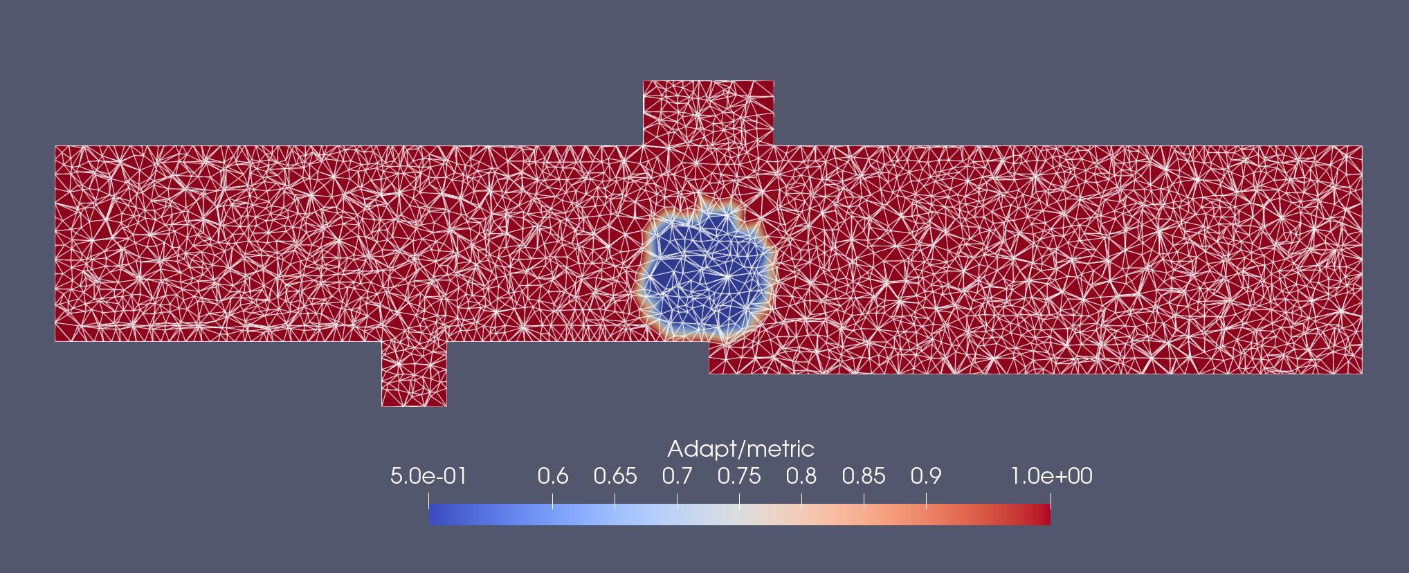
With this script , you can create a ball of value 0.5 in a uniform field of 1, as illustrated by the following figure:

Tubular exchanger x Reference “ball” field

Here we call the tekigo_sol.gatherscatter() method to get a GatherScatter object. This object loads the connectivity and how it behaves for different morphings.

gs = tekigo_sol.gatherscatter()
metric_field = gs.morph(metric_field,"smooth", passes=2)
tekigo_sol.evaluate_metric(metric_field)

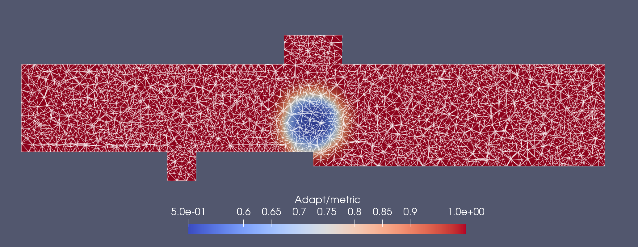
We ask then to GatherScatter the method .morph() for smoothing. passesis the number of times the action is applied. In short we apply here two gather/scatter:

Tubular exchanger x Two passes of “smooth” on the “ball” field

Dilate : propagate max. values

On the same reference field we can look what happens if in the gather/scatter we replace averaging by maximizing.

gs = tekigo_sol.gatherscatter()
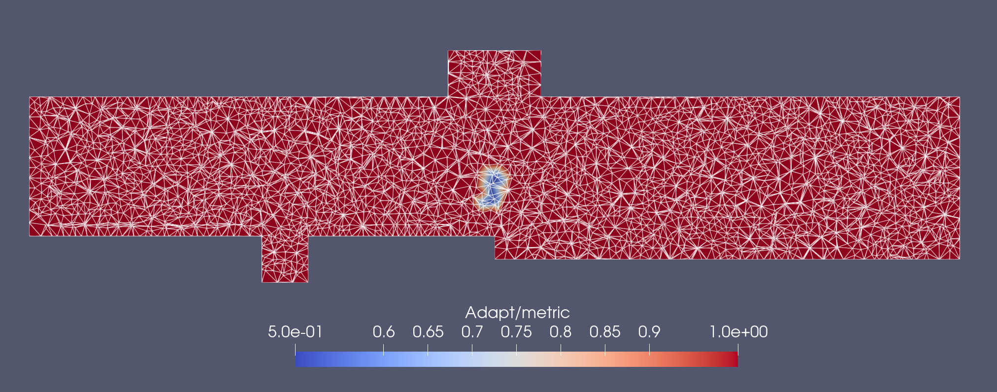
metric_field = gs.dilate(metric_field, passes=2)
tekigo_sol.evaluate_metric(metric_field)

Tubular exchanger x Two passes of “dilate” on “ball” field

This operation is particularly adapted to Y+ fields, propagating Y+ levels inside the domain and allowing more room for mesh adaptation

Erode : propagate min. values

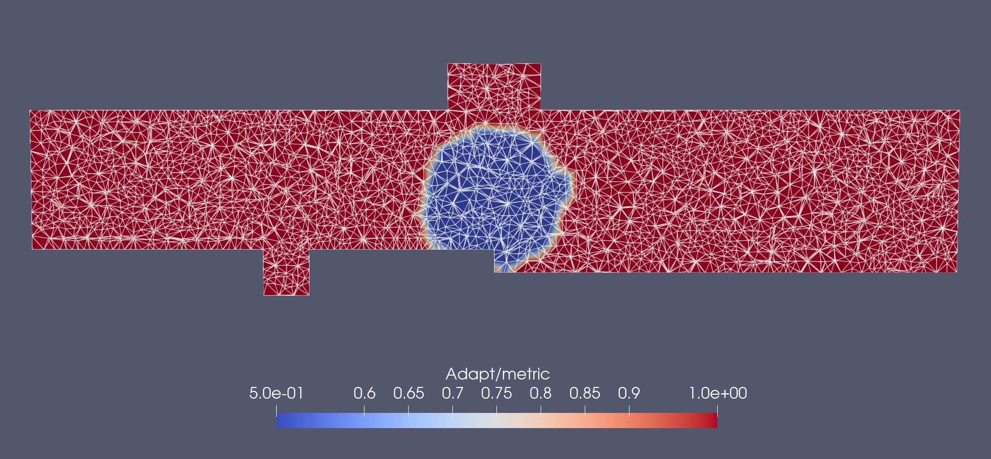
The opposite is erosion, where min values take precedence:

gs = tekigo_sol.gatherscatter()
metric_field = gs.erode(metric_field, passes=2)
tekigo_sol.evaluate_metric(metric_field)

Tubular exchanger x Two passes of “erode” on “ball” field

Advanced Combinations : Open and Close

Image treatments often use combinations of dilatations and erosions to clean imperfections.

open is first erode then dilate, or first min then max.
close is first dilate then erode, or first max then min.

To illustrate the action, we add a thin sheet of value 0.5 to the previous example:

import numpy as np
from tekigo import TekigoSolution

tekigo_sol = TekigoSolution(
    mesh='../../GILGAMESH/trapvtx/trappedvtx.mesh.h5',
    solution='combu.init.h5',
    out_dir='./Results')


x = tekigo_sol.load_qoi('/Mesh/coord_x')
y = tekigo_sol.load_qoi('/Mesh/coord_y')
z = tekigo_sol.load_qoi('/Mesh/coord_z')

x0 = 0.1
y0 = 0.105
z0 = 0.0

rad = np.sqrt((x-x0)**2+(y-y0)**2+(z-z0)**2)
metric_field = np.where(rad<0.01,0.5,1.0)

rad2 = np.sqrt((y)**2+(z)**2)
metric_field = np.where(abs(rad2-0.105)<0.001,0.5,metric_field)

The reference field looks like a porous sheet:

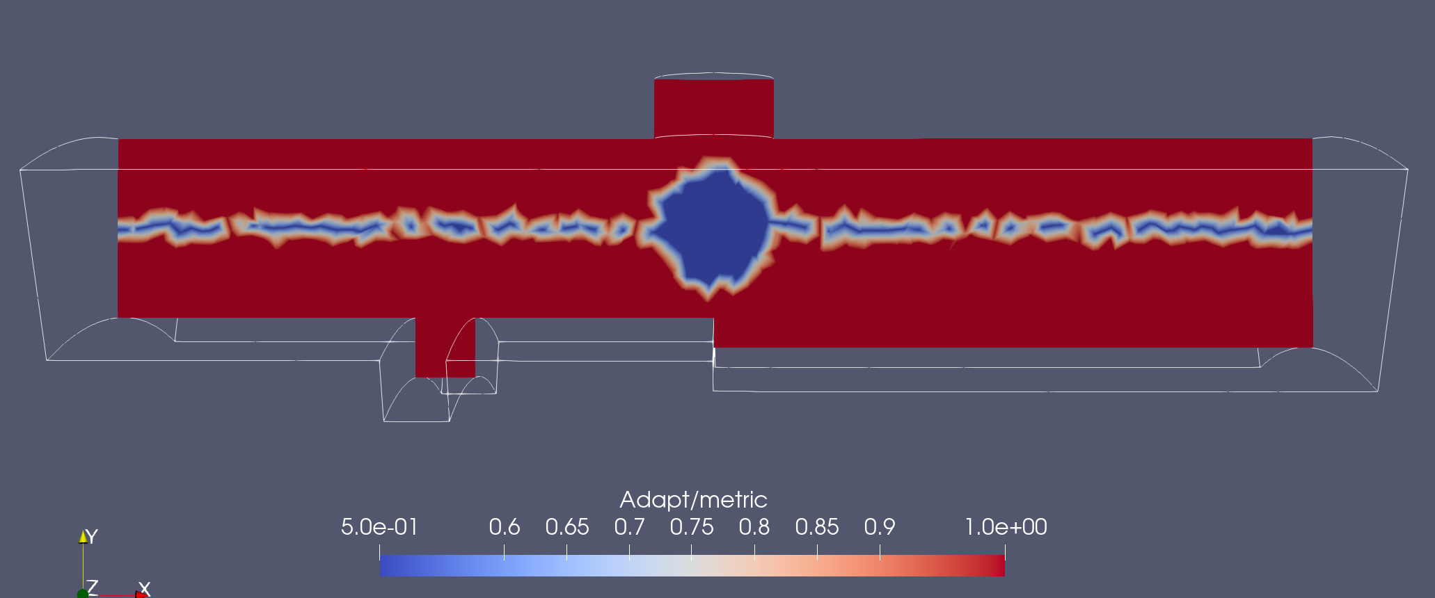x The reference “sheet” field

If we use open on this, the min values propagate, then recess. This “connects” the minimum values, without making the sheet or the ball thicker:

gs = tekigo_sol.gatherscatter()
metric_field = gs.open(metric_field, passes=2)
tekigo_sol.evaluate_metric(metric_field)

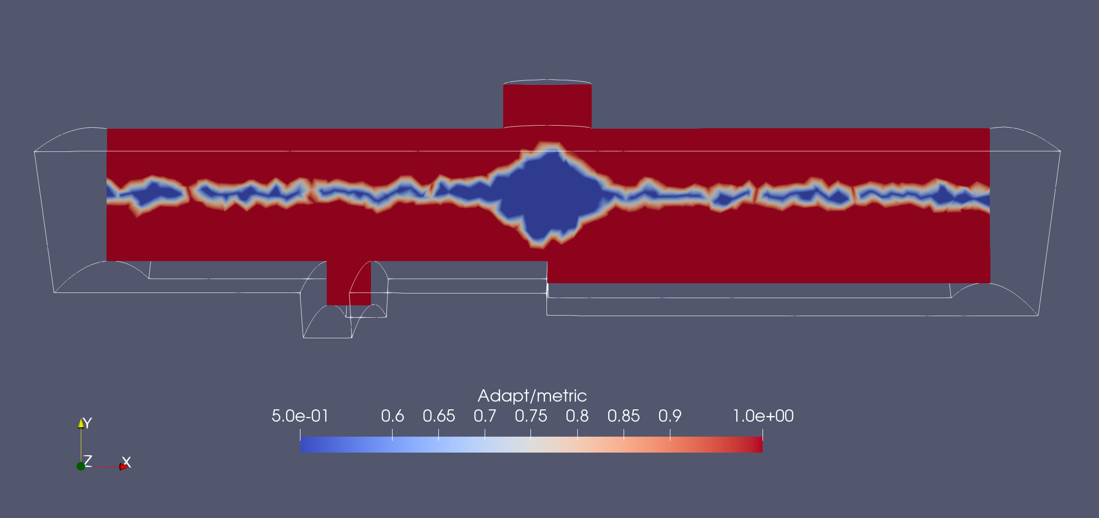x Applying 3 passes of “open” morphing to “sheet” field

On the other hand if we use close the sheet is removed but the ball stays in place. This “cleans” all spotty features. Meanwhile, large structures like the ball are unchanged.

gs = tekigo_sol.gatherscatter()
metric_field = gs.close(metric_field, passes=1)
tekigo_sol.evaluate_metric(metric_field)

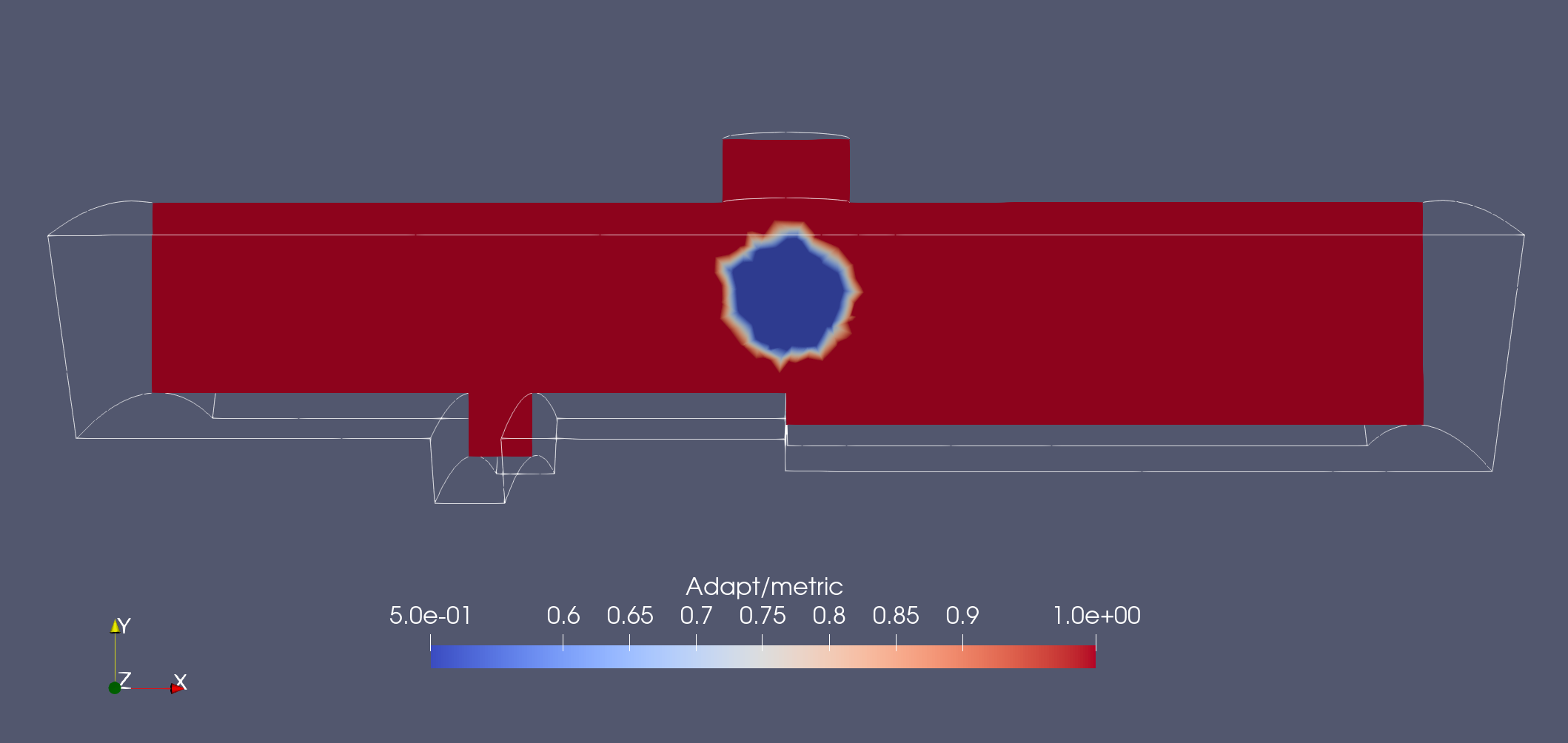x Applying 1 pass of “close” morphing to “sheet” field

Last remarks

The present example focuses on a metric, where the lowest values are the important ones. If you focus on a quantity of interest, the important values can be the maximum ones (heat release, Yplus). Therefore you may need to use the opposite function to get the expected action.

For exemple remove the spotiness of the field is close for a metric, but open for a positive source term.

The number of passes need may also vary depending on your cases. However, one pass means “one cell width” in all cases, which makes it quite easy to apprehend.